Customer Segmentation with Unsupervised Learning: A Complete Guide to Clustering Late-Paying Clients

Customer segmentation unsupervised learning is one of the most practical applications of machine learning for finance teams—and one of the most misunderstood. Most guides show you how to cluster customers by demographics or purchase frequency. But when your real problem is late payments eating into cash flow, you need a different approach entirely.

At Etere Studio, we've built segmentation models for clients managing anywhere from 200 to 15,000 accounts. The pattern is consistent: generic clustering tutorials don't translate to accounts receivable problems. The features that matter for payment behavior are different, the data structure requires careful aggregation, and the business interpretation of clusters determines whether the model actually gets used.

This guide walks through the complete process—from raw invoice data to actionable client personas that inform your collections strategy.

From Invoice-Level to Client-Level: Getting Your Data Structure Right

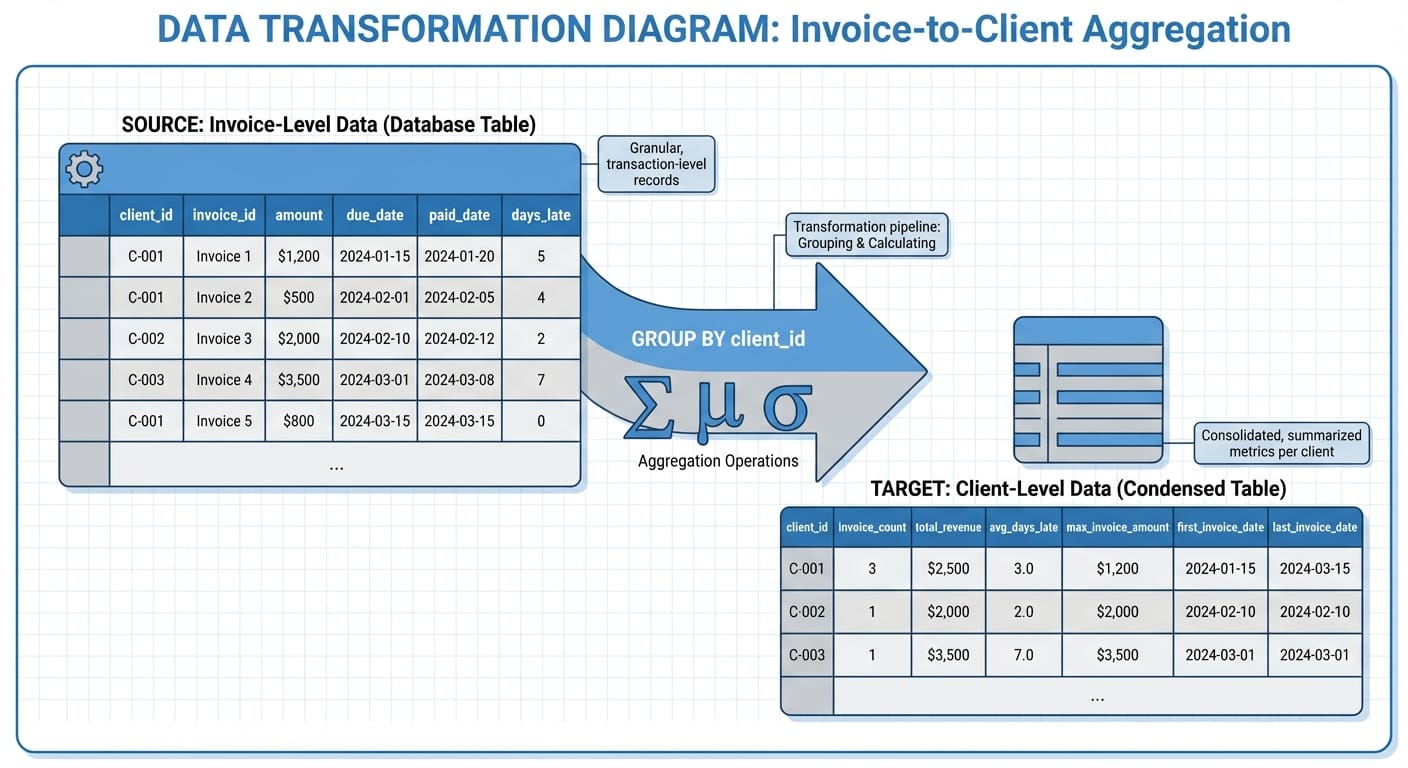
The first mistake teams make is clustering at the wrong level. Your ERP or accounting system stores data at the invoice level: one row per invoice, with dates, amounts, and payment status. But you're trying to understand clients, not invoices.

This means aggregation. And how you aggregate determines what patterns your model can find.

Here's the basic transformation:

import pandas as pd

# Starting with invoice-level data
# Columns: client_id, invoice_date, due_date, payment_date, amount, industry, company_size

client_df = invoices.groupby('client_id').agg({
    'invoice_id': 'count',
    'amount': ['sum', 'mean', 'std'],
    'days_past_due': ['mean', 'median', 'max', 'std'],
    'industry': 'first',
    'company_size': 'first'
}).reset_index()

client_df.columns = ['client_id', 'invoice_count', 'total_revenue', 
                     'avg_invoice_amount', 'invoice_amount_std',
                     'avg_days_past_due', 'median_days_past_due',
                     'max_days_past_due', 'days_past_due_std',
                     'industry', 'company_size']

The key insight: include both central tendency (mean, median) and dispersion (std, max) for payment timing. A client who averages 15 days late with low variance is very different from one who averages 15 days late but ranges from on-time to 90 days overdue.

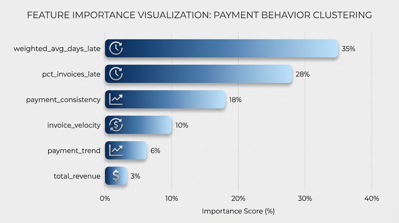
Feature Engineering: What Actually Predicts Payment Behavior

Raw aggregations are a starting point. The features that actually separate client segments come from domain knowledge about payment behavior.

Payment Timing Features

# Days past due is your core metric
client_df['days_past_due'] = (invoices['payment_date'] - invoices['due_date']).dt.days

# But you need more nuance
client_df['pct_invoices_late'] = invoices.groupby('client_id').apply(
    lambda x: (x['days_past_due'] > 0).sum() / len(x)
)

client_df['pct_severely_late'] = invoices.groupby('client_id').apply(
    lambda x: (x['days_past_due'] > 30).sum() / len(x)
)

# Payment consistency (coefficient of variation)
client_df['payment_consistency'] = (
    client_df['days_past_due_std'] / client_df['avg_days_past_due'].abs()
).fillna(0)

Invoice Velocity Features

How frequently a client transacts with you matters. High-volume clients who occasionally pay late present different risk than low-volume clients with the same late percentage.

# Invoice frequency (invoices per month)
client_df['invoice_velocity'] = client_df['invoice_count'] / months_in_period

# Recent trend - are they getting better or worse?
recent_avg = invoices[invoices['invoice_date'] > cutoff_date].groupby('client_id')['days_past_due'].mean()
historical_avg = invoices[invoices['invoice_date'] <= cutoff_date].groupby('client_id')['days_past_due'].mean()
client_df['payment_trend'] = recent_avg - historical_avg

Amount-Weighted Metrics

A client who pays small invoices on time but delays large ones behaves differently than one who's uniformly late. Weight your metrics by invoice amount:

def weighted_avg_days_late(group):
    return (group['days_past_due'] * group['amount']).sum() / group['amount'].sum()

client_df['weighted_avg_days_late'] = invoices.groupby('client_id').apply(weighted_avg_days_late)

# Exposure-at-risk: how much revenue is typically overdue
client_df['avg_overdue_exposure'] = invoices[invoices['days_past_due'] > 0].groupby('client_id')['amount'].mean()

Organizational Features

Incorporate what you know about the client beyond payment history:

# One-hot encode industry
industry_dummies = pd.get_dummies(client_df['industry'], prefix='industry')
client_df = pd.concat([client_df, industry_dummies], axis=1)

# Ordinal encode company size
size_map = {'small': 1, 'medium': 2, 'large': 3, 'enterprise': 4}
client_df['company_size_encoded'] = client_df['company_size'].map(size_map)

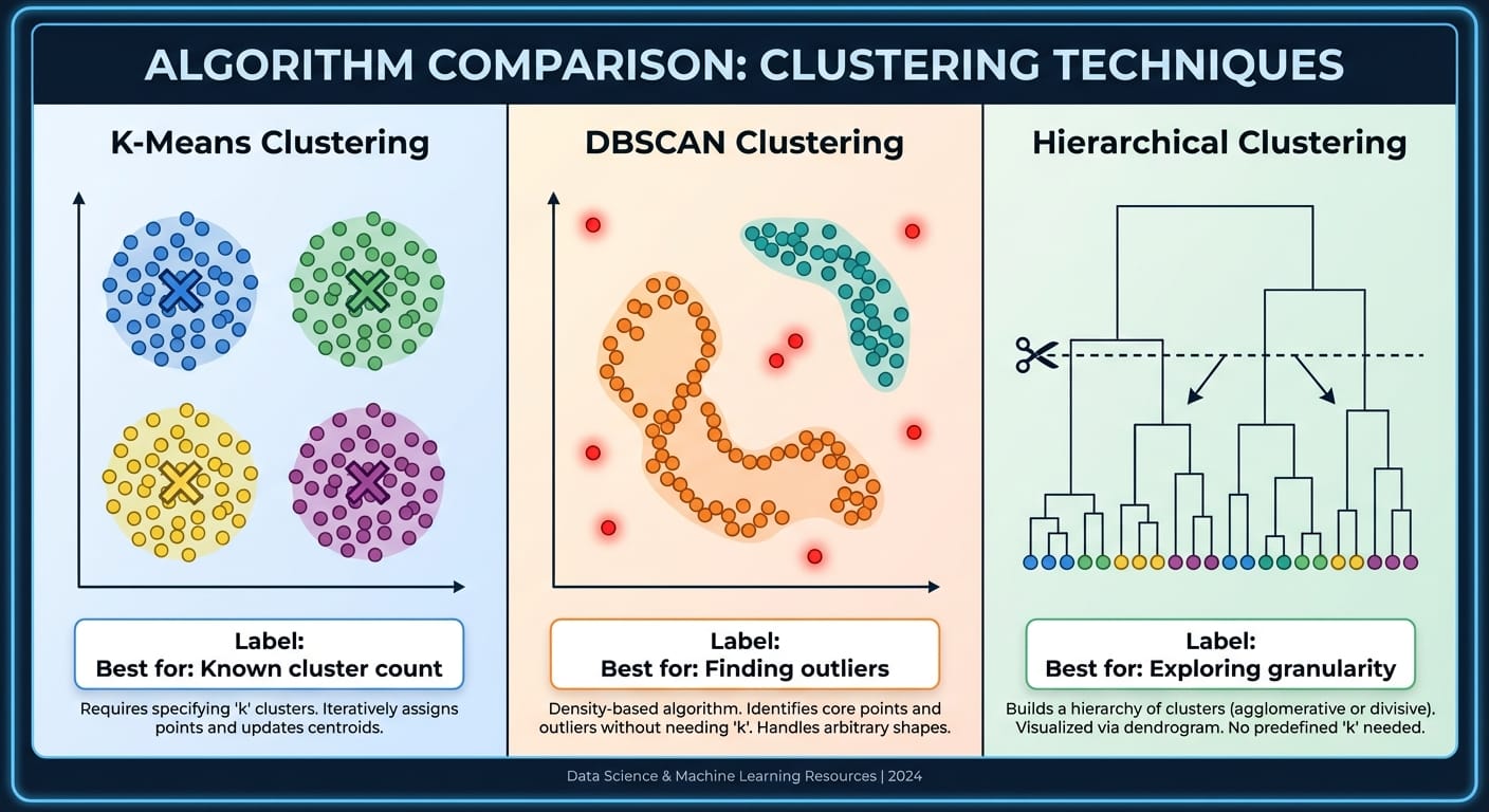
Choosing Your Clustering Algorithm

Three algorithms dominate customer segmentation unsupervised learning: K-Means, DBSCAN, and Hierarchical clustering. Each has tradeoffs that matter for payment behavior analysis.

K-Means: The Default Choice

K-Means works well when you expect roughly spherical clusters of similar size. For payment segmentation, this often holds—you typically get a "good payers" cluster, a "moderate risk" cluster, and a "high risk" cluster.

from sklearn.preprocessing import StandardScaler
from sklearn.cluster import KMeans

# Always scale features for K-Means
feature_cols = ['avg_days_past_due', 'pct_invoices_late', 'payment_consistency',
                'invoice_velocity', 'weighted_avg_days_late', 'total_revenue']

scaler = StandardScaler()
X_scaled = scaler.fit_transform(client_df[feature_cols])

# Fit K-Means
kmeans = KMeans(n_clusters=4, random_state=42, n_init=10)
client_df['cluster'] = kmeans.fit_predict(X_scaled)

Use K-Means when: You have a rough idea of how many segments you want, your features are numeric, and you need interpretable centroids.

DBSCAN: Finding Natural Groupings

DBSCAN doesn't require specifying the number of clusters upfront. It finds dense regions and labels sparse points as outliers—useful when you suspect your client base has natural groupings you haven't identified.

from sklearn.cluster import DBSCAN

dbscan = DBSCAN(eps=0.5, min_samples=10)
client_df['cluster'] = dbscan.fit_predict(X_scaled)

# Check how many outliers (-1 label)
print(f"Outliers: {(client_df['cluster'] == -1).sum()}")
print(f"Clusters found: {client_df['cluster'].nunique() - 1}")

Use DBSCAN when: You want to identify outliers explicitly, you don't know how many segments exist, or your clusters have irregular shapes.

Hierarchical Clustering: When Relationships Matter

Hierarchical clustering builds a tree of clusters, letting you choose the granularity after fitting. Useful when you want flexibility or need to explain the cluster structure to stakeholders.

from scipy.cluster.hierarchy import dendrogram, linkage, fcluster
import matplotlib.pyplot as plt

# Create linkage matrix
Z = linkage(X_scaled, method='ward')

# Visualize dendrogram to choose cut point
plt.figure(figsize=(12, 5))
dendrogram(Z, truncate_mode='level', p=5)
plt.title('Client Clustering Dendrogram')
plt.xlabel('Clients')
plt.ylabel('Distance')
plt.show()

# Cut at desired number of clusters
client_df['cluster'] = fcluster(Z, t=4, criterion='maxclust')

Use Hierarchical when: You need to present the clustering logic visually, you want to explore multiple granularity levels, or you have fewer than 10,000 clients (it doesn't scale well beyond that).

Evaluating Cluster Quality

Clustering has no ground truth, so evaluation is tricky. Use a combination of statistical metrics and business validation.

Statistical Metrics

Silhouette Score measures how similar points are to their own cluster versus other clusters. Ranges from -1 to 1; above 0.3 is decent, above 0.5 is good.

from sklearn.metrics import silhouette_score, silhouette_samples

score = silhouette_score(X_scaled, client_df['cluster'])
print(f"Silhouette Score: {score:.3f}")

# Per-cluster silhouette for diagnostics
silhouette_vals = silhouette_samples(X_scaled, client_df['cluster'])
for cluster in client_df['cluster'].unique():
    cluster_silhouette = silhouette_vals[client_df['cluster'] == cluster].mean()
    print(f"Cluster {cluster}: {cluster_silhouette:.3f}")

Elbow Method for K-Means helps choose the number of clusters:

inertias = []
K_range = range(2, 10)

for k in K_range:
    km = KMeans(n_clusters=k, random_state=42, n_init=10)
    km.fit(X_scaled)
    inertias.append(km.inertia_)

plt.plot(K_range, inertias, 'bo-')
plt.xlabel('Number of Clusters')
plt.ylabel('Inertia')
plt.title('Elbow Method')
plt.show()

Business Validation

Statistical metrics tell you if clusters are mathematically coherent. Business validation tells you if they're useful.

For each cluster, calculate:

cluster_summary = client_df.groupby('cluster').agg({
    'client_id': 'count',
    'total_revenue': 'sum',
    'avg_days_past_due': 'mean',
    'pct_invoices_late': 'mean',
    'weighted_avg_days_late': 'mean',
    'company_size_encoded': 'mean'
}).round(2)

cluster_summary.columns = ['client_count', 'total_revenue', 'avg_days_late',
                           'pct_late', 'weighted_days_late', 'avg_company_size']
print(cluster_summary)

Ask: Can your collections team describe each cluster in plain language? Do the clusters suggest different actions? If your finance team can't articulate what makes Cluster 2 different from Cluster 3, the segmentation isn't actionable.

Interpreting Clusters: Building Actionable Personas

The goal isn't pretty clusters—it's actionable personas that inform collections strategy. Here's what we typically find in late-payment segmentation:

Cluster 1: Reliable Payers (Low Risk)

• Average days past due: -2 to 5 (often pay early or on time)
• Percent invoices late: < 10%
• High payment consistency
• Action: Standard terms, low-touch collections, consider early payment discounts

Cluster 2: Occasional Offenders (Moderate Risk)

• Average days past due: 10-25
• Percent invoices late: 30-50%
• Variable consistency—some months fine, others delayed
• Action: Automated reminders at 7 and 14 days, personal outreach at 21 days

Cluster 3: Chronic Late Payers (High Risk)

• Average days past due: 30-60
• Percent invoices late: > 70%
• Often consistent in their lateness (they always pay, just late)
• Action: Shorter payment terms, deposits on large orders, proactive relationship management

Cluster 4: High-Value Problem Accounts

• Large companies with high revenue
• Moderate lateness but high exposure when late
• Often have complex approval processes
• Action: Dedicated account management, invoice format optimization, executive escalation paths

At Etere Studio, we've seen clients reduce their average DSO (Days Sales Outstanding) by 8-12 days after implementing cluster-specific collection strategies. The key is matching the intervention intensity to the cluster.

Putting It Into Production

A segmentation model that lives in a Jupyter notebook doesn't improve cash flow. Here's how to operationalize it:

1. Retrain quarterly — Payment behavior shifts. A client's cluster membership should update as new data arrives.
2. Build a scoring pipeline — New clients need cluster assignment based on early invoices. Use a simple rule-based fallback until you have enough history.
3. Integrate with your collections workflow — Export cluster assignments to your CRM or collections software. Tag accounts so your team knows the playbook.
4. Track outcomes by cluster — Measure collection rates, DSO, and write-offs per cluster. This validates your segmentation and identifies when it needs revision.

# Simple prediction for new clients with limited history
def assign_initial_cluster(new_client_features):
    # Scale using the same scaler
    scaled = scaler.transform([new_client_features])
    # Predict cluster
    cluster = kmeans.predict(scaled)[0]
    return cluster

Common Pitfalls

Overfitting to historical patterns — If your biggest late payer went bankrupt last year, their data shouldn't dominate your clusters. Consider recency weighting or excluding outliers.

Ignoring seasonality — Some industries pay late in Q4 due to budget cycles. Include month-of-year features or segment by season.

Too many clusters — Five to seven clusters is usually the practical maximum. More than that, and your team can't remember the playbook for each.

Forgetting the human element — Clusters are starting points. A longtime client who suddenly shifts to a high-risk cluster might be experiencing temporary difficulties, not a permanent change.

Customer segmentation unsupervised learning isn't magic—it's applied statistics with domain knowledge. The technical implementation matters less than asking the right questions: What features actually predict payment behavior? How will each segment change our collections approach? Can we explain these clusters to the finance team?

Get those answers right, and the clustering algorithm almost picks itself.

Building a payment behavior segmentation model for your business? We've helped finance teams implement these systems end-to-end. Let's talk